Our goal is to teach you how to solve systems of equations using matrix operations. This is an important section because we will go through elementary row operations and inverse matrices to solve bigger systems of equations. After Pre-Calculus, you might never see this until college.
Let's hack into the systems of equations using matrices. They are far easier to deal with in matrix form because we don't have to deal with all the variables until the end of each problem. In precalculus, it is most common to solve two or three variable systems of equations.
Just remember, two variable systems of equations solves for the intersection of the two functions. Three variable systems of equations solves for the intersections of three planes. Are you ready to enter the matrix? Or are you already there...
Sample Problem
Envision three planes in a 3-D space. They intersect at one point. We learned how to solve for the intersection of these in the previous section using Gaussian elimination. This is the same type of process but we are going to stay in matrices for a while. You are now part of the matrix whether you like it or not.
Our three planes are defined by the system of equations below:
2x + 8y + 4z = 26
x + 5y + 7z = 25
2x + 8y + 3z = 24
First let's put this in augmented matrix form.

Our goal will be to get the matrix in what we previously learned as triangular form (using Gaussian elimination). But since we are in a matrix, we'll call it row echelon form. The bottom line is that we want our matrix to look like this so that we can back-substitute values and solve for all three variables:

In order to get our augmented matrix into row echelon form, we will have to use elementary row operations on the matrix. You've done this before in Gaussian elimination.
It's elementary, my dear Watson. Here are the basic rules for elementary row operations:
Elementary Row Operations on Matrices
- You can switch any two rows of a matrix
- You can multiply an entire row by a non – zero number (or divide)
- You can add or subtract any row from another row even after a multiplication operation
Going back to our earlier problem, watch as we apply elementary row operations to change our augmented matrix into row echelon form. R1 stands for the current matrix Row 1. Each arrow will define row is getting changed for the next matrix (and what operations we did to get it).


Now, our matrix is in row echelon form! Back to our old system of equations. Now we know that z = 2 because if we switch back to equation form, it looks like this:
x + 4y + 2z = 13
y + 5z = 12
z = 2
Let's solve this equation now:
z = 2
y + 5(2) = 12
y = 2
x + 4(2) + 2(2) = 13
x + 12 = 13
x = 1
(1, 2, 2)
Sample Problem
3x + y + 4z = 13
4x + 2y + 8z = 24
2x + 10y + z = 4
Moving on to an even simpler method for solving a system of equations with matrices. This time we are going to put the matrix in reduced row echelon form which looks like this.

What is super cool about this method is that you will end up with x = #, y = #, and z = # eliminating the substitution method altogether.


The solution is (1, 2, 2)! Reduced echelon form is our favorite way to solve systems of equations.
Sample Problem
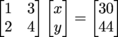
We promised to solve systems of equations with inverses and here it is. We'll start with this 2-D system:
1x + 3y = 30
2x + 4y = 44
We can set this a little bit different (kind of like reverse matrix multiplication):
Try to think of this as a simple little algebra problem like 2x = 10. To solve for x, you would need to divide each side by 2, or using fancy vocabulary, multiply each side by the inverse of 2 or 21. So what we would have is x = 10 × 2-11.
Using that logic, we shall solve this equation like this:
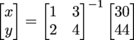
Using your previous knowledge (from Matrix Basix) of finding the inverse matrix, then multiplying, we get:
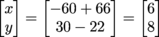
Our solution is (6, 8).