Electric Potential
We just had our minds blown adding up electric field contributions from multiple charges. More complicated electric fields must indicate complications elsewhere. Like how do continuous charge distributions affect the related quantities such as electric potential and flux? We’re about to find out. As a bonus, we’ll learn about the behavior of electric dipoles.
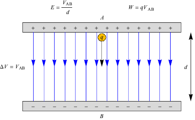
Let’s recall that the potential energy difference2 is the (negative) work done by a conservative force F when moving an object from point A to point B along a distance d, or ΔU = W = Fd. If we consider this potential energy per unit charge, and use the fact that F = qE, then we get the electric potential difference . Note that the potential is a scalar quantity without direction.
However, so that means that
  , where the charge Q remaining in the equation is of the point charge. Otherwise, we could calculate E from any of a host of equations derived (by calculus) from the shape the charges occupy.
In the case of the two electric plates shown in the diagram a ways above, the electric field is calculated by which is equivalent to
  by the definition of
  . Therefore the electric potential between two plates is
  .
.
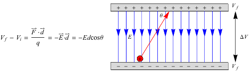
What if the charge moving within the uniform electric field is crossing it at an angle, as shown above? The change in voltage, then, is .It’s negative because of the work required to move a positive charge to a positive plate. But guess what? The same change in voltage applies to a straight vertical path as a slanted one.
It’s easy enough to calculate if d is just a straight line as it is in the diagrams with uniform electric fields above, or from one point charge to another but what if it’s not? Awesome—we sense more calculus to be spared from.
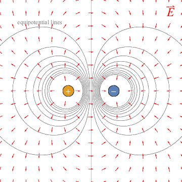
With our mathematical genius friend Mr. Calculus, adding up the cumulative electric potential on our behalf, we get the result of . That upside-down triangle thing is called a gradient, which sort of gives the three-dimensional slope of a line with x-, y-, and z-directions all taken into account. This is just an FYI. All we need to know for now though is that the electric field lines are perpendicular to lines of constant voltage, or equipotential lines.
This isn’t news: it was true in the last chapter too, as demonstrated by point charges’ fields and equipotential lines below. Aren’t they purty?
Also note that since the electric field E is in the same direction as the electric force, F, the lines of equipotential are not only perpendicular to the electric field, but also the force. Field, the force is with you.
Now let’s add two conditions to this. 1) E intersects the area at an angle θ, and 2) the surface is no longer a square. We guessed it: complicated conditions could bring calculus back into the picture. However, just as with an entirely enclosed point charge, as long as the area A encloses the total charge involved we still end up with , where
  is the charge within the enclosed area. Ringing any bells?
To use Gauss’ Law to advantage, we have to make sure E and A point in the same direction. This is why we have to pick a Gaussian surface appropriate to the problem. As we’ve seen before, the surface will most likely be a sphere with spherical symmetry, but cylindrical and plane symmetries might also be options.
For an example of spherical symmetry, let’s consider a charged sphere with uniform charge density for a total charge Q, with radius R. What’s the electric field beyond the sphere, for r > R?
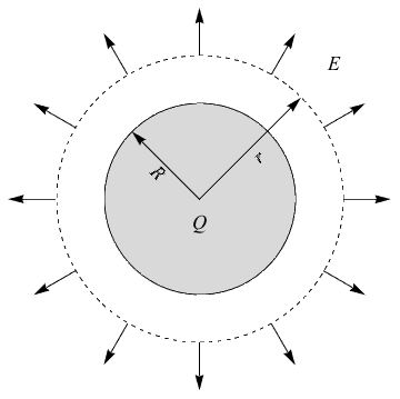
Gauss’ Law says . The enclosed charge is just Q for any radius larger than that of the sphere, so Qenc = Q, and A = 4πr2. Substituting in and solving for E we have
  . Why, that’s the same field as for a point charge! That makes sense, because for a radius larger than a charged sphere, the field from the sphere acts just the same as the field from a point charge.
Here’s an example of cylindrical symmetry, with our return to a single infinite metal plate. The area enclosed has some amount of charge determined by the charge density, .
.
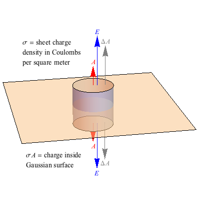
The cylinder we’re considering has 2 contributing areas of size A with the electric field pointing both directions. The sides don’t matter because they’re in line with E, so when we substitute in the values of E and A for Φ = EA and Aσ = Q for in Guass’ Law
  then we have
  which backs up the calculus derivation of
  for the electric field from an infinite charged plane from the last section.
An electric dipole consists of two opposite charges (± q) of equal magnitude held at a fixed distance d. When exposed to an electric field E, both charges feel a force F = ±qE which will cause them to rotate and align themselves with the field. The electric dipole moment p points from -q to +q and has a magnitude of p = qd. It’s an indication of polarity, akin to the rotational moment of inertia. Its direction matches the direction of d, as both are vector quantities. The following diagram summarizes this entire paragraph. Pictures are concise like that.
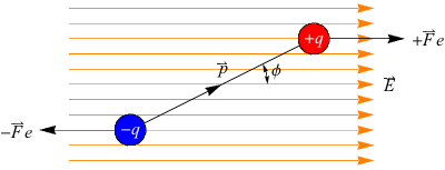
Since the forces are equal and opposite to each other, they add up to zero. However, the tendency of the dipole to align itself with the electric field E means there is a torque τ present on each charge as it rotates. Oh, yeah, torque. Torque is the rotational force. This torque is given by τ = p = E in vector form, with magnitude τ = pE sin ø = qEd sin ø taken out of vector form.
And why does anyone care about electric dipoles beyond curiosity’s sake? Well, because of the nature of molecules. Many, many molecules act as electric dipoles when in an electric field, and since electromagnetism is up there with gravity in importance, electric dipoles aren’t a rare thing. Any polar molecule, such as H2O, has an electric dipole moment.
Watch out for negative signs in electric potential and work calculations. They’re tricky.
Lastly, the angle involved in the electric dipole is defined with respect to the electric field lines, and not equipotential lines.
Section 1.2: Electric Potential
At the end of the section about electric fields we saw a diagram with a uniform electric fields and some references to work and electric potential. We need to talk about work and potential, so here it is again.Let’s recall that the potential energy difference2 is the (negative) work done by a conservative force F when moving an object from point A to point B along a distance d, or ΔU = W = Fd. If we consider this potential energy per unit charge, and use the fact that F = qE, then we get the electric potential difference
. Note that the potential is a scalar quantity without direction.However,
so that means that , where the charge Q remaining in the equation is of the point charge. Otherwise, we could calculate E from any of a host of equations derived (by calculus) from the shape the charges occupy.In the case of the two electric plates shown in the diagram a ways above, the electric field is calculated by
which is equivalent to by the definition of . Therefore the electric potential between two plates is .What if the charge moving within the uniform electric field is crossing it at an angle, as shown above? The change in voltage, then, is
.It’s negative because of the work required to move a positive charge to a positive plate. But guess what? The same change in voltage applies to a straight vertical path as a slanted one.It’s easy enough to calculate if d is just a straight line as it is in the diagrams with uniform electric fields above, or from one point charge to another but what if it’s not? Awesome—we sense more calculus to be spared from.
With our mathematical genius friend Mr. Calculus, adding up the cumulative electric potential on our behalf, we get the result of
. That upside-down triangle thing is called a gradient, which sort of gives the three-dimensional slope of a line with x-, y-, and z-directions all taken into account. This is just an FYI. All we need to know for now though is that the electric field lines are perpendicular to lines of constant voltage, or equipotential lines. This isn’t news: it was true in the last chapter too, as demonstrated by point charges’ fields and equipotential lines below. Aren’t they purty?
Also note that since the electric field E is in the same direction as the electric force, F, the lines of equipotential are not only perpendicular to the electric field, but also the force. Field, the force is with you.
Gauss’ Law
We learned earlier the electric flux ΦE is simply a measure of how many electric field lines pass through a surface area3. In fact, if the electric field E passes through a square of area A perpendicularly, then ΦE = EA. If it doesn’t, we use EA cos θ. And if the electric field lines pass straight through one side of the area to the other, then flux is zero because the same number of lines go in as go out.Now let’s add two conditions to this. 1) E intersects the area at an angle θ, and 2) the surface is no longer a square. We guessed it: complicated conditions could bring calculus back into the picture. However, just as with an entirely enclosed point charge, as long as the area A encloses the total charge involved we still end up with
, where is the charge within the enclosed area. Ringing any bells?To use Gauss’ Law to advantage, we have to make sure E and A point in the same direction. This is why we have to pick a Gaussian surface appropriate to the problem. As we’ve seen before, the surface will most likely be a sphere with spherical symmetry, but cylindrical and plane symmetries might also be options.
For an example of spherical symmetry, let’s consider a charged sphere with uniform charge density for a total charge Q, with radius R. What’s the electric field beyond the sphere, for r > R?
Gauss’ Law says
. The enclosed charge is just Q for any radius larger than that of the sphere, so Qenc = Q, and A = 4πr2. Substituting in and solving for E we have . Why, that’s the same field as for a point charge! That makes sense, because for a radius larger than a charged sphere, the field from the sphere acts just the same as the field from a point charge.Here’s an example of cylindrical symmetry, with our return to a single infinite metal plate. The area enclosed has some amount of charge determined by the charge density,
.The cylinder we’re considering has 2 contributing areas of size A with the electric field pointing both directions. The sides don’t matter because they’re in line with E, so when we substitute in the values of E and A for Φ = EA and Aσ = Q for
in Guass’ Law then we have which backs up the calculus derivation of for the electric field from an infinite charged plane from the last section.Electric Dipoles
We’ll end this section with a quick introduction to the electric dipole. Electric dipole, meet Shmoop students. Shmoop students, electric dipole.An electric dipole consists of two opposite charges (± q) of equal magnitude held at a fixed distance d. When exposed to an electric field E, both charges feel a force F = ±qE which will cause them to rotate and align themselves with the field. The electric dipole moment p points from -q to +q and has a magnitude of p = qd. It’s an indication of polarity, akin to the rotational moment of inertia. Its direction matches the direction of d, as both are vector quantities. The following diagram summarizes this entire paragraph. Pictures are concise like that.
Since the forces are equal and opposite to each other, they add up to zero. However, the tendency of the dipole to align itself with the electric field E means there is a torque τ present on each charge as it rotates. Oh, yeah, torque. Torque is the rotational force. This torque is given by τ = p = E in vector form, with magnitude τ = pE sin ø = qEd sin ø taken out of vector form.
And why does anyone care about electric dipoles beyond curiosity’s sake? Well, because of the nature of molecules. Many, many molecules act as electric dipoles when in an electric field, and since electromagnetism is up there with gravity in importance, electric dipoles aren’t a rare thing. Any polar molecule, such as H2O, has an electric dipole moment.
Common Mistakes
Gauss’ Law has spared many the student the headache of deriving the electric field of some continuous charge distribution by calculus. It’s there to help.Watch out for negative signs in electric potential and work calculations. They’re tricky.
Lastly, the angle involved in the electric dipole is defined with respect to the electric field lines, and not equipotential lines.