Magnetic Fields
Now, it’s time to jump into the different but similar world of magnetism. We’ve already learned a bit about magnetic fields, magnets, polarity, the Lorentz force with charged particles moving in a magnetic field, electromagnetic radiation, and the electromagnetic spectrum4. What’s missing?
So far in this unit we’ve studied stationary charges that have constant electric fields, which is known as electrostatics. Magnetostatics, on the other hand, deal with steady currents that create constant magnetic fields as well as the ferromagnetic materials which produce constant magnetic fields. We’ve talked enough about those before, though, so we turn our attention to the magnetic fields created by currents of electricity.
The stage is set with wires running thither and yon with magnetic fields running in circles around them….
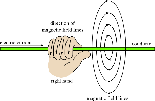
We find the direction the right-hand rule: the thumb points in the direction of the current, with the fingers wrapping around the imaginary wire, indicating the direction of the magnetic field around the wire.
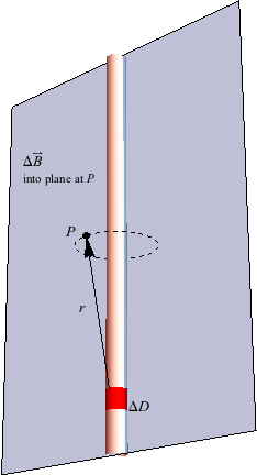
Two French scientists, Jean Baptiste Biot and Félix Savart, managed to solve the problem of the magnitude of the magnetic field, probably over a bottle of Bordeaux and some stinky cheese. In the following diagram, we have a magnetic field contribution, pointing into the page at point P, and current and length on the plane of the page. This field contribution is perpendicular to both the current element IΔd and the vector distance r between Point P and IΔd.
Finding B then becomes a calculus problem—hooray—in which the distance r is continuously changing. Let’s pause to celebrate skipping the math.
The Biot-Savart equation is used for any geometrical configuration and, just as we saw with electric fields, to arrive at various equations for these varied geometric configurations. The results of a few of these configurations from Biot-Savart are included below. . Here µo is called the permeability of free space and is equal to
  .
.
Well, who knows…maybe it’ll come up during a trivia night.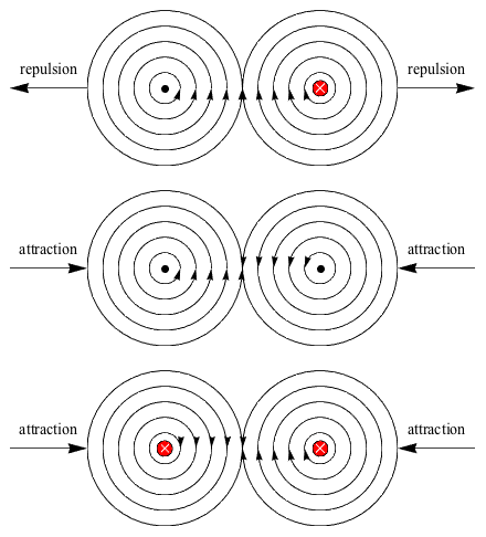
There are three cases for two parallel, current-carrying-but-not-card-carrying wires. The dots in the image represent the wire coming out of the page, while the x’s in the image represent the wire going into the page. That way we can see the magnetic field lines around them. If the two currents move in the same direction, the magnetic force between them is attractive. Sadly, not for the pair of wires traveling in opposite directions. They don’t want to be anywhere near each other.
This could be a good science experiment for those with circuit equipment nearby.
Anyways, the individual fields of each wire are calculated by the same equation as stated above, . Then the force per unit length of wire is determined by
  . That’s because F = qvB is equivalent to F = ILB. The per time rate changes from a velocity to a current, leaving distance by itself.
The force direction requires the old right hand rule, where we stick the pointer finger along the current direction, curl our other fingers to the direction of the magnetic field, then stick the thumb up in the direction of the force. They’re all perpendicular to each other. Try it: use the three cases shown above to practice the right hand rule.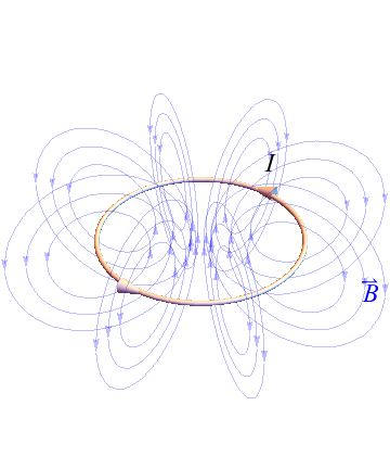
In a ring, the magnetic field point either inward or outward depending on the direction the current flows in the loop. If the current loop is on the plane of this page and traveling counter-clockwise, then the magnetic field in the center of the loop is out of the page. Use the right hand rule taught earlier to find this, at any point (and every point) on the loop. Its magnitude is calculated by where r is the radius of the loop. 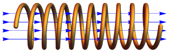
Just as electric field , a magnetic field has magnetic field lines. We’ve drawn them before. And just as there’s electric flux, there’s magnetic flux. It’s a twin equation: , or for a field perpendicular to the normal of the cross sectional area, ΦB = BA. Let’s take a step back. With Gauss’ Law, we stated that
  . If the enclosed charge is a dipoleor other net neutral object, then Qenc = 0 and the electric flux ΦE is zero as well. Analogously, if there were a single magnetic “charge,” this enclosed charge would be proportional to the total magnetic flux.
But wait a second. There’s no such thing as a magnetic monopole. They come in pairs with north and south poles—even a broken magnet has a north and a south pole. Magnetic field lines must form continuous loops. Therefore, the equation reduces to ΦB = BA = 0 for any closed surface, regardless of whether or not there are currents creating magnetic fields.
The presence of any magnetic field guarantees that any enclosed area has any many lines going in as out and that magnetic flux is zero. Good to know. For trivia.
Ampere’s Law allows us to equate the magnetic field in terms of current, thanks to calculus we get to skip over. First, the person using calculus finds a line of constant magnetic field, such as the circle around a straight wire, on which to add up a loop of distance. Then, by adding up all the bits of length around a loop of a total length we’ll call d, we relate the enclosed current to the magnetic field. In its most general form, Ampere’s Law is Bd = μ0Ienc, and it can be applied for conductors of any shape.
For a path of a circle around one straight conducting wire with current I, the path d is the circumference 2πr so Bd = μ0Ienc becomes B(2πr) = μ0I, which leads us straight back to the field we found with Bio-Savart, .
.
If we chose another shape such as a current loop or a solenoid, we’d once again arrive at the same conclusion as Biot-Savart. Just as with the electric field and electric flux, we have two methods to finding the respective fields. Backup.
For example, Ampere’s Law applied to a solenoid of length L says that BL = μ0NI. Then, since , B = μ0nI. What did we tell ya? Biot-Savart and Ampere’s Law produce the same equations.
The bigger trick is in knowing which is easier to use, but since we’re not responsible for calculus in this course, we’re spared the decision. We win.
Remember that a moving point charge does NOT produce a constant magnetic field. We need to consider current distributions in order to apply the laws of magnetostatics.
So far in this unit we’ve studied stationary charges that have constant electric fields, which is known as electrostatics. Magnetostatics, on the other hand, deal with steady currents that create constant magnetic fields as well as the ferromagnetic materials which produce constant magnetic fields. We’ve talked enough about those before, though, so we turn our attention to the magnetic fields created by currents of electricity.
The stage is set with wires running thither and yon with magnetic fields running in circles around them….
The Biot-Savart Law
We just learned about using calculus to find the electric field of a continuous charge distribution by adding up all the contributions from each charge individually. Surely, the equivalent exists in the world of magnetism? How do we relate the magnitude of a magnetic field B to the current I that produces it?We find the direction the right-hand rule: the thumb points in the direction of the current, with the fingers wrapping around the imaginary wire, indicating the direction of the magnetic field around the wire.
Two French scientists, Jean Baptiste Biot and Félix Savart, managed to solve the problem of the magnitude of the magnetic field, probably over a bottle of Bordeaux and some stinky cheese. In the following diagram, we have a magnetic field contribution, pointing into the page at point P, and current and length on the plane of the page. This field contribution is perpendicular to both the current element IΔd and the vector distance r between Point P and IΔd.
Finding B then becomes a calculus problem—hooray—in which the distance r is continuously changing. Let’s pause to celebrate skipping the math.
The Biot-Savart equation is used for any geometrical configuration and, just as we saw with electric fields, to arrive at various equations for these varied geometric configurations. The results of a few of these configurations from Biot-Savart are included below.
Magnetic Field Around a Single Wire with a Current
A particularly useful magnetic field equation to know is the magnetic field at a distance a from a long straight wire with current I as shown in the diagram above This is given by. Here µo is called the permeability of free space and is equal to .Well, who knows…maybe it’ll come up during a trivia night.
Magnetic Field Two infinite wires
There are three cases for two parallel, current-carrying-but-not-card-carrying wires. The dots in the image represent the wire coming out of the page, while the x’s in the image represent the wire going into the page. That way we can see the magnetic field lines around them. If the two currents move in the same direction, the magnetic force between them is attractive. Sadly, not for the pair of wires traveling in opposite directions. They don’t want to be anywhere near each other.
This could be a good science experiment for those with circuit equipment nearby.
Anyways, the individual fields of each wire are calculated by the same equation as stated above,
. Then the force per unit length of wire is determined by . That’s because F = qvB is equivalent to F = ILB. The per time rate changes from a velocity to a current, leaving distance by itself.The force direction requires the old right hand rule, where we stick the pointer finger along the current direction, curl our other fingers to the direction of the magnetic field, then stick the thumb up in the direction of the force. They’re all perpendicular to each other. Try it: use the three cases shown above to practice the right hand rule.
Magnetic Field in the Middle of a Current Loop
In a ring, the magnetic field point either inward or outward depending on the direction the current flows in the loop. If the current loop is on the plane of this page and traveling counter-clockwise, then the magnetic field in the center of the loop is out of the page. Use the right hand rule taught earlier to find this, at any point (and every point) on the loop. Its magnitude is calculated by
where r is the radius of the loop. Magnetic Field in a Solenoid
Just as electric field , a magnetic field has magnetic field lines. We’ve drawn them before. And just as there’s electric flux, there’s magnetic flux. It’s a twin equation:
, or for a field perpendicular to the normal of the cross sectional area, ΦB = BA. Let’s take a step back. With Gauss’ Law, we stated that . If the enclosed charge is a dipoleor other net neutral object, then Qenc = 0 and the electric flux ΦE is zero as well. Analogously, if there were a single magnetic “charge,” this enclosed charge would be proportional to the total magnetic flux.But wait a second. There’s no such thing as a magnetic monopole. They come in pairs with north and south poles—even a broken magnet has a north and a south pole. Magnetic field lines must form continuous loops. Therefore, the equation reduces to ΦB = BA = 0 for any closed surface, regardless of whether or not there are currents creating magnetic fields.
The presence of any magnetic field guarantees that any enclosed area has any many lines going in as out and that magnetic flux is zero. Good to know. For trivia.
Ampere’s Law
We weren’t lying up there when we said things would get easier. Turns out the equivalent of Gauss’ Law exists for continuous currents as well, ensuring that the magnetic flux remains zero through the area. Thank goodness.Ampere’s Law allows us to equate the magnetic field in terms of current, thanks to calculus we get to skip over. First, the person using calculus finds a line of constant magnetic field, such as the circle around a straight wire, on which to add up a loop of distance. Then, by adding up all the bits of length around a loop of a total length we’ll call d, we relate the enclosed current to the magnetic field. In its most general form, Ampere’s Law is Bd = μ0Ienc, and it can be applied for conductors of any shape.
For a path of a circle around one straight conducting wire with current I, the path d is the circumference 2πr so Bd = μ0Ienc becomes B(2πr) = μ0I, which leads us straight back to the field we found with Bio-Savart,
.If we chose another shape such as a current loop or a solenoid, we’d once again arrive at the same conclusion as Biot-Savart. Just as with the electric field and electric flux, we have two methods to finding the respective fields. Backup.
For example, Ampere’s Law applied to a solenoid of length L says that BL = μ0NI. Then, since
, B = μ0nI. What did we tell ya? Biot-Savart and Ampere’s Law produce the same equations. The bigger trick is in knowing which is easier to use, but since we’re not responsible for calculus in this course, we’re spared the decision. We win.
Common Mistakes
Again, just as for electric fields, make sure the situation described matches the equation chosen. So many parallels. And then again, so many perpendiculars. Remember the right hand rule works only with the right hand.Remember that a moving point charge does NOT produce a constant magnetic field. We need to consider current distributions in order to apply the laws of magnetostatics.