Sample Problem
Sketch a rough graph of  .
.
We're jumping right into this with a sample problem, because we know that we can handle it. Everything we've been looking at has prepared us for graphing, even a beast like this degree 9 polynomial.
As you might be able to guess, we want as much information as we can get on the roots of this polynomial; we've only spent a few thousand words talking about them. Not that we're obsessed with them or anything.
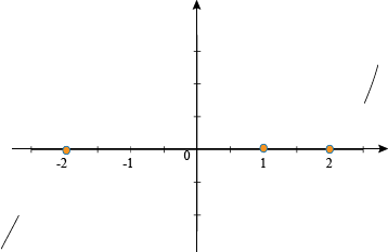
That's because the roots are where the action is when graphing polynomials. This time we have the roots laid out for us: x = -2, 1, and 2. Let's double-check that we have them all, though. If we missed one, would we have egg on our face or what?
According to the Fundamental Theorem of Algebra, there are 9 roots total, but they can be real or complex. Looking at our roots, they have multiplicities of 3 + 4 + 2 = 9. That means the roots we have are all the roots that exist. At least, all the ones that exist in this universe. We make no promises about Universe B.
The multiplicity at x = 1 is odd, so it will pass through the x-axis, flexing just a little, while x = -2 and 2 will tap the axis but stay on the same side.
One last thing we need to know is the end behavior of the polynomial. We're not talking about how they dance, but how the "arms" at the far ends of the graph point.
The polynomial has a degree of 9, which is odd, so one end points up and the other points down. To see which is which, we have to look at the sign of the leading coefficient.
Multiplying the first terms of each factor gets us  . This is positive, so the polynomial starts off pointing down to the left and points up on the right side of the graph. It points the same as y = x3, but not nearly as stylishly.
Now we start sketching our graph.
We start off by getting our ends on the page. Hey, stop snickering.
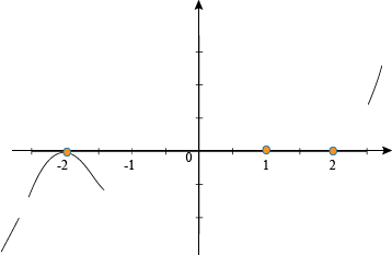
We need to pick a zero at one end of the graph to start working from. Going from the left, we have x = -2, which we know will just touch the x-axis, but not cross over. The graph is negative before we reach x = -2, so that means that the graph will continue to be negative afterwards as well. Aw, come on graph, cheer up. We'll have you finished up in no time.
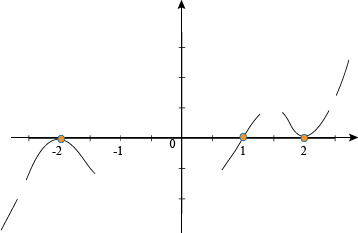
We keep working our way to the right in the same way. The graph is still negative, but it crosses over at x = 1. The even multiplicity at x = 2 means the polynomial glides down, taps the axis, then swings back up while staying positive. At this point, it will stay positive forever and ever and ever. We wanted you to cheer up, graph, but isn't this a bit excessive?
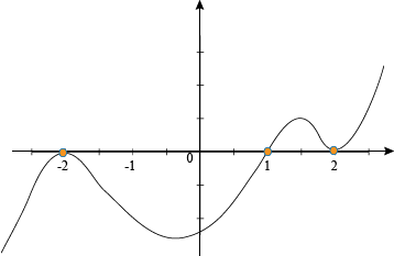
Now we can connect all of our parts together into a full graph of the polynomial. Don't worry too much about the swoops and dips on the graph. No one is going to blame you if it goes a little high or low. Well, we won't blame you, at least. If it really worries you, feel free to plot a few points, like the y-intercept, to make the graph more accurate.
The most important thing, though, is getting the zeros graphed correctly, the behavior of the graph near each one, and then the overall shape of things in between. If we really want to know exactly how far down the graph goes between -2 and 1, for instance, we can plug numbers into the original equation and find out that way.
Sample Problem
Sketch a rough graph of y = x3 + x2 − 5x + 3.
Not every polynomial is given to us nicely factored out. Sometimes we have to track down the zeros ourselves. At least we're accomplished root finders. We can take some time off from tending the potato farm to track down some polynomial roots.
Descartes has a lunch appointment in 30 minutes, so we'll use his Rule of Signs first so he can make his date. For y = f(x), the sign changes twice, so we have 2 or 0 positive real roots. Now we can look at f(-x):
(-x)3 + (-x)2 – 5(-x) + 3
= -x3 + x2 + 5x + 3
The sign only changes once in the front, so we have 1 or 0 negative real roots. Catch you later, Descartes.
The next step is to find possible rational roots for the polynomial, and to start checking them. The Rational Root Theorem will probably be faster than asking people on the street if they've seen any roots. The factors in the numerator are ±1 and ±3, and we only have ±1 to deal with in the denominator. So, our possible rational roots are ±1 and ±3.
We'll start by testing 1. Not only is it easy to plug into a polynomial, but we have two possible chances to potentially catch a real root, according to Descartes' sign. It also says, "Eat at Joe's." Guess he decided to sell advertising space.

Ring the bell, we have a root. If we hadn't found one, we could have used the quotient from the synthetic division to test if x = 1 was an upper bound, but we don't have to. We can instead find the factorization of the original polynomial and x – 1.
y = x3 + x2 − 5x + 3 = (x – 1)(x2 + 2x – 3)
Now we have a defenseless quadratic equation in our clutches. We know lots of ways to deal with them. We can factor them with our eyes closed. We can factor them in our sleep. We can factor them after we've died and become a spooky ghost.
y = (x – 1)(x + 3)(x – 1)
= (x – 1)2(x + 3)
From here, we're in the same spot we were in for the first problem. That was a long and winding road to reach here. We have roots of -3 and 1, with multiplicities of 1 and 2 respectively.
We again have an odd polynomial with a positive leading coefficient. The end behavior is left arm down and right arm up.
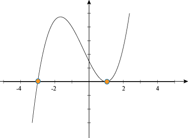
At x = -3, the graph passes right through, negative to positive, without any flexing. Lines just don't work out. At x = 1, it starts positive and stays positive after touching the x-axis, then shoots off for the stars.
So hey, we just had a scary thought. What do we do if the polynomial only has complex roots? Sorry, buster, but then you have to painstakingly plug and chug points in, making sure not to miss any bumps along the graph. It is no fun at all.